Software and Methods for Forming Process Simulation
Lecture 2 · Modelling and Simulation of Processes I – Forming (MSPO2_6I)
Winter semester 2026/2027
Faculty of Materials Science and Technology · STU Bratislava

Closed-die forging of a yoke simulated in DEFORM-3D (© SFTC)
Questions that forming simulation answers
- Will the die cavity fill? — underfill, laps, folds, piping
- What press do I need? — force and energy versus stroke
- Will the part crack or neck? — damage, FLD, thinning
- Will it keep its shape? — springback, warpage, distortion
- What will the tool life be? — stress, wear, temperature
- What is inside? — grain size, phases, hardness

Sequence of several rolling passes in DEFORM-3D (© SFTC)
Where today's lecture fits
- Lecture 1: modelling, model types, the modelling chain
- Lecture 2 (today): methods and software that solve the model
- Lecture 3: material models — flow stress, hardening
- Lectures 4–6: preprocessing, sheet and bulk forming examples
- Lab sessions: DEFORM — so today's Part III is your toolkit for the whole semester
Today's agenda (120 min)
| Time | Block | Content |
|---|---|---|
| 0 – 10 | Introduction | Motivation, context, agenda |
| 10 – 25 | I · Analytical methods | Slab method, upper bound, slip lines; solving in MATLAB / Python / GAMS |
| 25 – 67 | II · Forming software | 1 Ansys Forming · 2 Simufact Forming · 3 Abaqus · 4 Moldflow |
| 67 – 97 | III · DEFORM | Main part — the software of our lab sessions |
| 97 – 112 | IV · Special simulation software | Overview · simple examples · use cases |
| 112 – 120 | Summary and questions | Key takeaways, review questions |
Part I — Analytical Methods of Forming
Closed-form and semi-analytical models: fast, transparent and the reference for every FEM result
Classical analytical methods of plasticity theory
| Method | Principle | Typical output | Typical process |
|---|---|---|---|
| Slab method (elementary theory) | Force equilibrium on a thin slab; homogeneous deformation | Pressure distribution, force | Upsetting, forging, rolling, drawing |
| Slip lines | Characteristics of the stress field, rigid-perfectly plastic material, plane strain | Exact stress field, force | Indentation, extrusion, machining |
| Upper bound (UBM, UBET) | Kinematically admissible velocity field; minimum power | Force ≥ actual, die filling | Extrusion, closed-die forging |
| Lower bound | Statically admissible stress field | Force ≤ actual | Limit analysis |
| Visioplasticity | Measured grid deformation → strain rates → stresses | Experimental flow field | Extrusion and forging research |
- Common assumptions: rigid-plastic material, constant (or mean) flow stress σf, simple friction law, simple geometry
Drawing and extrusion: closed-form results
Sachs (slab method) — wire drawing stress
- \(\alpha\) die semi-angle, \(A_0, A_1\) cross-section before and after
- Condition: \(\sigma_d \le \sigma_f\) ⇒ maximum reduction per pass
Upper bound — extrusion pressure
- \(R_{ext}=A_0/A_1\) extrusion ratio, \(\alpha\) die semi-angle
- The shear term grows with α, the friction term falls ⇒ optimum die angle → optimisation problem
Solving analytical models: MATLAB · Python · GAMS
| Problem type | Forming example | Tool |
|---|---|---|
| Closed form | Drawing force, Sachs stress | NumPy · MATLAB |
| Nonlinear equation | Neutral point in rolling | fzero · brentq |
| Differential equation | Slab-method forging, von Kármán | ode45 · solve_ivp |
| Symbolic computation | Deriving slab-method equations | SymPy · Symbolic TB |
| Optimisation NLP | Upper bound, optimum angle | fmincon · GAMS/CONOPT |
| MINLP | Pass schedule, number of passes | GAMS/BARON · Pyomo |
| Framework | Groove rolling | PyRolL (TU Freiberg) |
# Upsetting force – slab method (Python)
import numpy as np
from scipy.integrate import quad
sf, mu = 250.0, 0.2          # MPa, -
R0, h0 = 10.0, 30.0          # mm
for h in np.linspace(30, 10, 5):
    R = R0*np.sqrt(h0/h)     # volume constancy
    p = lambda r: sf*np.exp(2*mu*(R-r)/h)
    F = quad(lambda r: p(r)*2*np.pi*r, 0, R)[0]
print(f"h={h:5.1f} mm F={F/1e3:7.1f} kN")Why analytical methods are not enough
| Aspect | Analytical methods | Numerical software (FEM / FVM) |
|---|---|---|
| Geometry | Simple (cylinder, strip, cone) | Arbitrary 3D from CAD |
| Material | Constant or mean σf | σf(φ, φ̇, T), anisotropy, damage |
| Output | Force, mean pressure | Full fields: strain, T, stress, defects, microstructure |
| Time to answer | Seconds | Minutes to days |
| Transparency | Every term is visible | "Black box" — must be checked |
- Use analytical results for the first estimate and to check FEM results — leave the rest to the software
Part II — Forming Simulation Software
1 Ansys Forming · 2 Simufact Forming · 3 Abaqus · 4 Moldflow → 5 DEFORM (Part III)
Two groups of forming software
Dedicated process-oriented
- Templates: presses, tools, draw beads, passes
- For the process engineer, not the FEM specialist
- Sheet: Ansys Forming, AutoForm, PAM-STAMP
- Bulk: Simufact, DEFORM, QForm, FORGE
- Plastics: Moldflow, Moldex3D
General-purpose nonlinear FEM
- The user builds everything: parts, contacts, steps
- Maximum flexibility, user subroutines (UMAT)
- Abaqus, LS-DYNA, Ansys Mechanical, MSC Marc
- Research, teaching, unusual processes
| Solver type | Principle | Where |
|---|---|---|
| Implicit (static) | Equilibrium in every increment, large steps | DEFORM, Abaqus/Standard, springback |
| Explicit (dynamic) | Small stable time steps, robust contact | LS-DYNA (Ansys Forming), Abaqus/Explicit |
| Finite volumes (Euler) | Fixed mesh, material flows through it | Simufact FV, Moldflow solvers |
Every program follows the same workflow
- Steps 1–4 = preprocessing (lecture 4)
- Step 6 = postprocessing (lectures 5–6)
- Programs differ mainly in how much of steps 1–4 their templates automate
- "Garbage in, garbage out": the quality of the answer is set by the flow curve and the friction coefficient
Ansys Forming — stamping with the LS-DYNA solver
- Complete application for sheet metal stamping: pre-, solution and postprocessing in one environment
- Solver: LS-DYNA explicit (implicit for gravity and springback)
- Vendor: Ansys, part of Synopsys since 2025; first version 2022 R1
- Project types: cold and hot stamping (press hardening), hemming (beta), One Step (inverse method)
- For process engineers and tool makers — no need to be an FEM expert
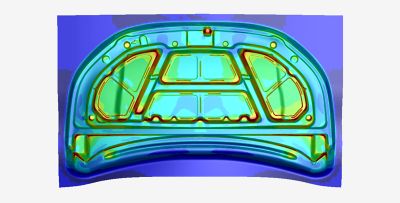
Car hood inner panel in Ansys Forming (© Ansys / Synopsys)
Workflow and typical results
| Result | Answers |
|---|---|
| FLD, formability index | Crack or wrinkle? |
| Thinning | Local thickness loss |
| Springback | Shape after unloading |
| Stoning, zebra | Visible surface defects |
| Draw-in, skid marks | Blank movement |
| Press force | Press size |
- Rule: 3 elements on a 90° radius
- Presets: Fast · Accurate · Very Accurate
Video: Ansys Forming — stamping from start to finish
Simufact Forming — two solvers in one program
- Process-oriented software for bulk and sheet metal forming; Simufact (Hamburg) → MSC → Hexagon
- Forging, cold heading, extrusion, ring rolling, open-die forging, fine blanking, self-pierce riveting, clinching, heat treatment
| Finite elements (FE) | Finite volumes (FV) | |
|---|---|---|
| Description | Lagrangian — the mesh moves with the material | Eulerian — fixed mesh, material flows through the cells |
| Mesh | Hexahedra, tetrahedra, remeshing | No remeshing needed |
| Suited for | Cold forming, sheet metal, tool stress, joining | 3D hot closed-die forging with flash |
| Origin | MSC Marc solver | MSC SuperForge |
- Switching FE ↔ FV between operations; FV parallelised in 2022 — up to 4× faster
Simufact Forming — defect prediction

a) "Flow defect zones": detection of piping and folds (© Hexagon)
b) Damage-based crack initiation and propagation (© Hexagon)
- Piping and folds: typical in forging and extrusion — hard to predict without simulation
- Damage-based separation: 2D mesh splitting, 3D element deletion — blanking, fine blanking, riveting
Video: fold formation in forging a fork head
Abaqus — the general-purpose tool
- Dassault Systèmes SIMULIA; Abaqus/CAE and 3DEXPERIENCE; free Learning Edition (≈ 1000 nodes)
- No forming templates: the user builds parts, contacts and steps — flexible, ideal for research (UMAT/VUMAT)
| Abaqus/Explicit | Abaqus/Standard | |
|---|---|---|
| Use | Forming with complex contact, large deformations | Springback, smooth quasi-static loading, heat transfer |
| Strength | Robust contact, no convergence problems | True equilibrium, large increments |
| Watch out for | Small stable time step → mass scaling | Convergence with contact |
Abaqus example: axisymmetric deep drawing of a cup
- Part — blank: deformable axisymmetric shell; punch, die, blank holder: analytical rigid
- Property — steel, E = 200 GPa, ν = 0.3, flow curve
- Step — Dynamic, Explicit, 0.007 s
- Interaction — penalty friction μ = 0.1 (die, blank holder)
- Load — punch 60 mm, Smooth Step amplitude
- Mesh — blank only, refined at the radii
- Results — PEEQ, thickness STH, punch force

Deep drawing results in Abaqus/CAE (© CAE Assistant)
Abaqus: large deformations and damage
| Technique | Use |
|---|---|
| ALE adaptive meshing | Forging, rolling, extrusion (Explicit) |
| Adaptive remeshing | Error-driven (Standard) |
| Mesh-to-mesh mapping | Very large deformations, forging operations |
| CEL (Euler) | Extreme material flow |
- Damage: ductile, Johnson-Cook, shear, FLD, FLSD, MSFLD, M-K
- Springback: ≥ 5–7 integration points through the thickness, kinematic hardening

ALE adaptive meshing in Abaqus/Explicit (© TECHNIA)
Autodesk Moldflow — forming of polymers
- Founded 1978 in Melbourne (Colin Austin); Autodesk since 2008; current version 2027
- Adviser (designers) · Insight (analysts) · Synergy interface · Communicator viewer
- Physics: non-Newtonian viscous melt flow + heat transfer — not solid plasticity
- Viscosity: Cross-WLF · PVT: Tait equation
- ≈ 13,900 thermoplastics in the database
Moldflow: mesh types and defects
| Mesh | Principle | Use |
|---|---|---|
| Midplane 2.5D | Shells on the mid-surface; Hele-Shaw | Thin walls, fastest |
| Dual Domain 2.5D | Matched meshes on both surfaces | Thin simple parts |
| 3D tetrahedra | Full 3D flow, no Hele-Shaw | Thick, massive parts |
| 1D beam | Line elements | Runners and cooling channels |
| Defect | Remedy suggested by simulation |
|---|---|
| Short shot | Add/move gate, thicker wall, hotter melt |
| Weld lines | Move the gate to a non-critical area |
| Air traps | Venting, gate change |
| Sink marks | Core out thick sections, longer packing |
| Warpage | Balance cooling, uniform wall |
- Analysis sequence: gate location → fill → pack → cool → warp (+ fibre orientation → structural FEM)
Video: Autodesk Moldflow overview
Comparison of the five programs
| Aspect | Ansys Forming | Simufact | Abaqus | Moldflow | DEFORM |
|---|---|---|---|---|---|
| Focus | Sheet metal stamping | Bulk, sheet, joining | General-purpose FEM | Plastic injection moulding | Bulk, HT, microstructure |
| Solver | LS-DYNA explicit | FE (Marc) + FV | Standard + Explicit | Flow (2.5D / 3D) | Implicit Lagrangian, ALE |
| Setup | Templates | Templates | Manual | Templates | Templates + open |
| Strength | Springback compensation | Fast FV hot forging | Flexibility, UMAT | Fill, pack, cool, warp | Remeshing, microstructure, wear |
| Vendor | Synopsys | Hexagon | Dassault Syst. | Autodesk | SFTC (USA) |
- There is no "best" software — only software suited to the process and the question
Part III — DEFORM
Design Environment for FORMing — the software of our lab sessions
DEFORM — from ALPID to a complete process simulator
- FEM system for forming, heat treatment, machining and joining
- Vendor: SFTC, Columbus, Ohio (≈ 30 people)
- Roots: ALPID at Battelle (U.S. Air Force) — the first practical FEM tool for production forming
- Theory: Kobayashi, Oh & Altan, Metal Forming and the FEM (1989)
| Year | Milestone |
|---|---|
| 1989 | DEFORM-2D |
| 1991 | SFTC founded, takes over DEFORM |
| 1993 | DEFORM-3D |
| 2024 · 2025 | V14.0 · V14.1 |
| 2026 | V14.1.1; V15.0 announced |
Yoke forging — DEFORM-3D (© SFTC)
The DEFORM product family
| Product | What it is |
|---|---|
| DEFORM-2D | Axisymmetric and plane problems — our first lab sessions |
| DEFORM-3D | Full 3D deformation, temperature and microstructure |
| DEFORM PREMIER | All systems and modules in one package |
| FORMING EXPRESS | Simplified system for forging, heading, extrusion, drawing |
| DEFORM-HT | Heat treatment: carburising, quenching, tempering |
| DEFORM-3D Machining | Turning, drilling, milling templates; tool wear (Usui) |
| Modules | Microstructure, DOE/optimisation, ring rolling, open-die forging, shape rolling, extrusion |
- Processes: forging (hot/warm/cold), rolling, extrusion, drawing, heading, tube piercing, spinning, blanking, riveting, clinching, powder compaction, shot peening
The DEFORM solver: rigid-viscoplastic formulation
- \(\bar\sigma, \dot{\bar\varepsilon}\) effective stress and strain rate · \(K\) penalty constant (incompressibility) · \(F_i\) surface tractions
- The unknowns are velocities → Newton-Raphson / direct iteration in every step (implicit, updated Lagrangian)
- Elastic strains are neglected — suited to large plastic flow (forging); elasto-plastic option for springback, residual stresses, tools
- ALE and steady-state solvers for ring rolling, shape rolling, extrusion, tube piercing
Working with DEFORM: Pre → Simulation → Post
| Object type | Meaning |
|---|---|
| Rigid | Non-deforming tools (optionally with heat transfer) |
| Plastic | Workpiece, rigid-viscoplastic |
| Elastic | Tool stress analysis |
| Elasto-plastic | Springback, residual stresses |
| Porous | Powder, sintered material |
- Machine models: hydraulic, mechanical, screw press, hammer (energy)
Key inputs: flow stress, friction, heat transfer
- Tabulated data from the material library (steels, Al, Ti, superalloys, Cu …) or from your own compression tests
- Neural-network prediction of flow stress from chemical composition (V13+)
| Conditions | Friction factor m |
|---|---|
| Cold, good lubrication | 0.08 – 0.12 |
| Warm | ≈ 0.2 |
| Hot forging, lubricated | 0.3 |
| Hot forging, dry | 0.7 – 1.0 |
- Die–workpiece heat transfer coefficient; the Inverse HTC module derives it from thermocouples
- Most sensitive inputs: flow stress and friction
Automatic remeshing and multiple operations
- The Lagrangian mesh deforms with the material → automatic remeshing when an element degenerates or penetrates the tool
- Tetrahedra (3D), quadrilaterals (2D), optionally hexahedra; mesh windows refine critical regions
- Each remeshing interpolates state variables → keep the number of remeshings reasonable (volume loss)
Multiple Operations (MO) — one chain, runs automatically
Results: from die filling to tool life
- Die filling, laps and folds, flow lines (point tracking, flow net)
- Effective strain, strain rate, temperature, triaxiality
- Force–stroke curve, energy → press selection
- Tool stress (elastic dies, prestressing) and tool wear
- ≈ two dozen ductile damage models, element deletion
Normalised Cockcroft–Latham criterion
Archard tool wear
σ₁ maximum principal stress · p pressure · v sliding velocity · H tool hardness
Microstructure and heat treatment
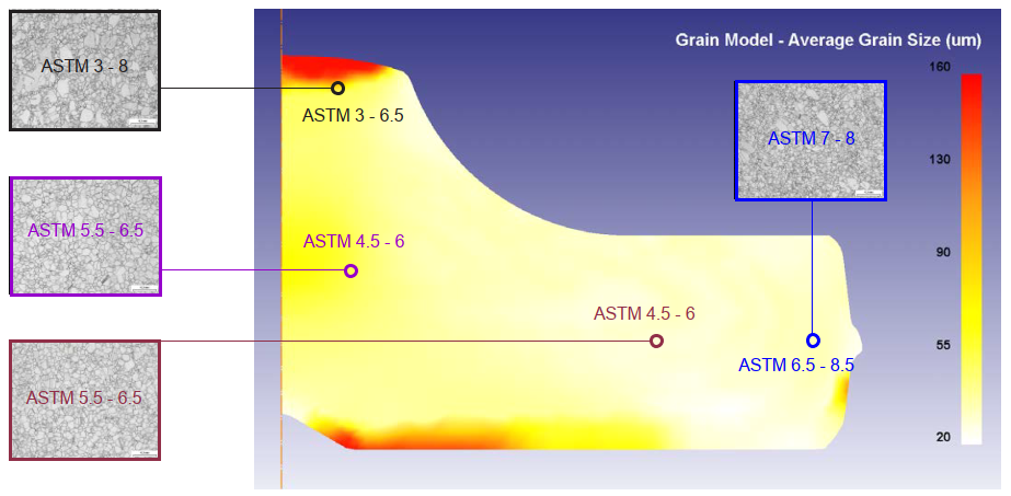
a) Grain size in a forged Waspaloy turbine disc (© SFTC)
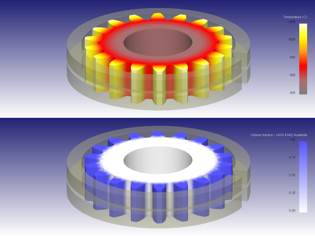
b) Induction-hardened spur gear (© SFTC)
- Dynamic / static recrystallisation, grain growth, phase fractions, hardness, precipitates, texture (crystal plasticity)
Video: DEFORM — simulation of metal forming processes
Video: forged turbine disc — microstructure simulation
DEFORM today: V14.1 → V15.0 (User Group Meeting, May 2026)
| Area | New feature | Benefit |
|---|---|---|
| Solver | Stiffness reuse for elastic objects (MUMPS + ESE) | 1.2 – 2.9× faster with elastic tools |
| Solver | Iterative elasto-plastic solver EPCG, MPI | > 50 % faster than CG |
| Spinning | QEM + partial domain | 14 min instead of 17 – 35 h |
| AI | U-Net surrogate model for multi-pass shape rolling + CMA-ES groove optimisation | Design in seconds |
| Quenching | CFD boiling model (vapour film, nucleate boiling) | Realistic HTC |
| Blanking | 3D mesh in the clearance zone and its remeshing | Fine mesh only in the clearance |
| Automation | Python DEFORM-API, PPTX report generation | Scripting, machine learning |
DEFORM in our lab sessions
- Bring: your notes from Part I (the slab method formula)
- Check as you go: is the force realistic? was the volume preserved? how many remeshings were there?
- Assessment: assignment 20 pts + written exam 80 pts
Part IV — Special Simulation Software
Beyond Lagrangian FEM: inverse methods, finite volumes, particles, discrete elements, multiscale and data-driven tools
Methods and the software that implements them
| Method | Principle | Software (examples) | Use in forming |
|---|---|---|---|
| Inverse one-step | Unfolding the finished part into a plane | AutoForm OneStep, Ansys Forming One Step, PAM-STAMP | Blank shape, quick feasibility |
| Finite volumes | Fixed Eulerian mesh | Simufact FV, QForm Extrusion* | Hot forging, Al extrusion |
| SPH (particles) | Meshless Lagrangian particles | DualSPHysics, LS-DYNA SPH | Extreme deformations, MIM, FSW |
| DEM | Contact of discrete grains | EDEM, LIGGGHTS, Yade | Powder die filling |
| Multiscale | CA, crystal plasticity, phase field | DAMASK, DEFORM Microstructure | Recrystallisation, texture, earing |
| Data-driven | ANN / ROM trained on FEM | Python (PyTorch), DEFORM-API | Springback, rolling design |
| Analytical frameworks | Coupled analytical models | PyRolL | Rolling pass design |
| Physical simulation | Reproducing φ, φ̇, T on a specimen | Gleeble | Flow curves, validation |
A simple example: one extrusion, four descriptions
Schematic: how different methods discretise material flow through a die
Simple examples: inverse method and AI surrogate model
Inverse one-step (sheet metal)
- Minutes instead of hours; ignores process history
Surrogate model (bulk forming)
- Valid only within the trained design space
Use cases from research and industry
| Problem | Approach | Result |
|---|---|---|
| Closed-die forging of a rib-web part | UBET + plasticine experiments | Force and flow agree with the physical model |
| Extrusion of Al profiles, ratio > 25 | FVM on an Eulerian mesh (+ ANN/GA) | No remeshing; optimised die parameters |
| Metal powder injection moulding (17-4 PH) | SPH in DualSPHysics | Verified by real injections |
| Powder die filling (Distaloy AE) | DEM → density as input to compaction FEM | Filling shoe design before trials |
| Earing in deep drawing of AA 5754 | Crystal plasticity FEM | Ears predicted from texture |
| Grain size in hot forging | Cellular automata coupled with DEFORM-2D | Recrystallised fraction and grain size |
| Springback in bending | ANN trained on FEM | Fast springback for new cases |
Video: dedicated extrusion simulation (QForm)
Summary
- Analytical methods (slab method, upper bound, slip lines) give a quick force estimate and are the first check of every FEM result
- Dedicated software automates the process: Ansys Forming (stamping), Simufact (bulk + joining), Moldflow (polymers)
- General-purpose FEM (Abaqus) is flexible, but the user builds everything
- DEFORM: implicit rigid-viscoplastic FEM, automatic remeshing, damage, tool wear, microstructure — our tool for the lab sessions
- Special software goes beyond the limits of FEM: FVM, SPH, DEM, inverse and multiscale methods, AI surrogate models
Next time: material models — elasticity, plasticity, hardening, flow curves
Review questions
- Why is the contact pressure in upsetting highest in the centre? What increases this peak?
- Upper bound force: is it greater or smaller than the actual one — and why is that useful?
- Explicit vs. implicit solver: which for stamping, which for springback?
- What is the difference between the Lagrangian (FE) and the Eulerian (FV) description?
- Why is the physics in Moldflow different from that in DEFORM?
- Which two inputs in DEFORM affect the result most? What is the friction factor m?
- Name one damage model and one wear model in DEFORM and what they predict.
- When would you use the inverse one-step method or an ANN surrogate instead of full FEM?
References and further reading
- Necpal, M.; Sobota, R.: Modelovanie a simulácia procesov tvárnenia. Spektrum STU, 2023 (in Slovak)
- Kobayashi, S.; Oh, S.I.; Altan, T.: Metal Forming and the Finite Element Method. Oxford UP, 1989
- Hosford, W.F.; Caddell, R.M.: Metal Forming: Mechanics and Metallurgy. Cambridge UP
- Dixit, P.M.; Dixit, U.S.: Modeling of Metal Forming and Machining Processes. Springer, 2010
- Bílik, J.; Kapustová, M.; Ridzoň, M.: Teória tvárnenia. AlumniPress, 2015 (in Slovak)
- SFTC: DEFORM brochures, DEFORM News 2022–2025, UGM Spring 2026 — deform.com
- Ansys Forming User's Guide 2026 R1 — ansys.synopsys.com
- Hexagon: Simufact Forming 2021.1 and 2022 — nexus.hexagon.com
- Abaqus Analysis User's Manual; TECHNIA and CAE Assistant tutorials
- Autodesk Moldflow help, What's New 2025–2027 — autodesk.com
- Weiner et al.: PyRolL, JOSS 9(93), 2024
Images and videos © their owners, referenced for teaching purposes